Statistical analysis colouring-based
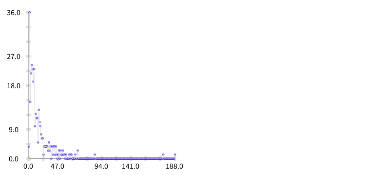
First of all I want to build an histogram of the metric values to understand better their distribution. I implemented the following code to do that:
bag := Bag new.
RTObject withAllSubclasses do:[:e| bag add: e numberOfMethods].
res := ((0 to: bag max) collect:[:v| v @ (bag select:[:va| va = v]) size ]).
    b := RTGrapher new.
    b extent: 300 @ 300.

    ds := RTDataSet new.
    ds dotShape ellipse color: (Color blue alpha: 0.5).
    ds points: (0 to: bag max).
    ds connect.
    ds y: [ :v | (res select:[:va| va x = v ]) first y ].
    b add: ds.

    b axisXWithNumberOfTicks: 10.
    b axisYWithNumberOfTicks: 10.
b build.
The result is shown in the picture below:
The next step is to build a function that approximates to these data. In consequence I built a polynomial regression (using the least square method) thanks to the SciSmalltalk project. To load SciSmalltalk do:
Gofer new
    url: 'http://www.smalltalkhub.com/mc/SergeStinckwich/SciSmalltalk/main';
    package: 'ConfigurationOfSciSmalltalk';
    load.
(Smalltalk at: #ConfigurationOfSciSmalltalk) loadDevelopment.
Therefore, the code below uses it to build the approximation.
|estimation|

fit := DhbPolynomialLeastSquareFit new:8.
bag := Bag new.
RTObject withAllSubclasses do:[:e| bag add: e numberOfMethods].
(0 to: bag max)
    do:[:v| fit add: (DhbWeightedPoint
        point: v @ (bag select:[:va| va = v]) size) ].
estimation := fit evaluate.

b := RTGrapher new.
b extent: 300 @ 300.

ds := RTDataSet new.
ds dotShape ellipse color: (Color blue alpha: 0.5).
ds points: (0 to: bag max).
ds connect.
ds y: [ :v | estimation value: v ].
b add: ds.

b axisXWithNumberOfTicks: 10.
b axisYWithNumberOfTicks: 10.
b build.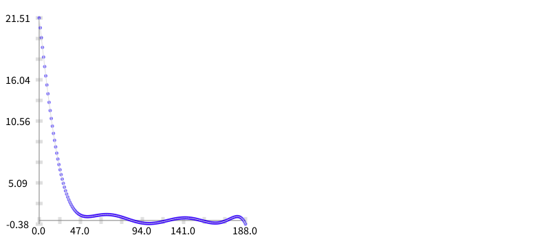
Now we can use the polynomial function with a standard metric normaliser. The code below applied this idea to the original visualisation:
|estimation|
fit := DhbPolynomialLeastSquareFit new:8.
bag := Bag new.
RTObject withAllSubclasses do:[:e| bag add: e numberOfMethods].
(0 to: bag max)
do:[:v| fit add: (DhbWeightedPoint
point: v @ (bag select:[:va| va = v]) =size) ].
estimation := fit evaluate.
v := RTView new.
objs := RTObject withAllSubclasses.
els := RTBox new height:#numberOfMethods; color:[Color red]; elementsOn: objs.
v addAll: els.
RTEdgeBuilder new
view: v;
objects: objs from: [ :entry | entry superclass ].
RTMetricNormalizer new
elements: els;
normalizeColor: #numberOfMethods
using: {Color black . Color green . Color black}
using:[:v| estimation value: v ].
RTTreeLayout on: els.
els @ RTPopup.
v @ RTDraggableView.
v open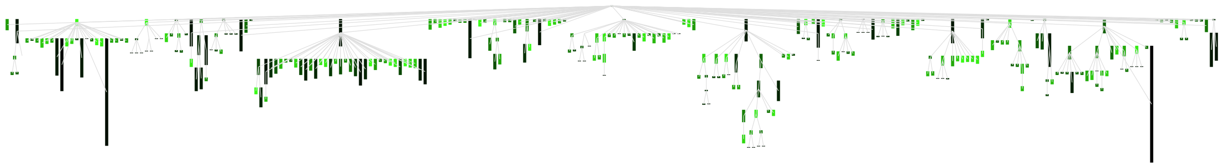 Right-click on the image and open it in a new window for a larger picture
The following animated GIF (@http://gifmaker.cc) shows the differences between the original approach and the statistical based one.
 Right-click on the image and open it in a new window for a larger picture
Statistical-based approach characteristics:
- It does take into account distribution of metric values.
- Useful for detecting distant values from 'the center'
- Not too useful for finding maximum values
This approach seems more useful if highlighting the median.
The following code implements a visualisation clustering the values in four quartiles (assigning different intensities of green) and highlights the nodes that match one of the values splitting the quartiles (including the median).
v := RTView new.
objs := RTObject withAllSubclasses.
nums := objs collect: #numberOfMethods.
median := nums median.
median2 := (nums reject:[:e| e < median]) median.
median1 := (nums reject:[:e| e > median]) median.
els := RTBox new
    height: [ :e | e numberOfMethods ];
    color: [ :e |
        e numberOfMethods < median1
            ifTrue: [Color green]
            ifFalse: [
                e numberOfMethods <= median
                ifTrue: [ Color r: 0 g: 0.75 b: 0 ]
                ifFalse: [
                    e numberOfMethods <= median2
                    ifTrue:[Color r: 0 g: 0.5 b: 0 ]
                    ifFalse:[Color r: 0 g: 0.25 b: 0] ] ]];
        borderColor:[:e|
            ((Array with: median with: median1 with: median2)
                    includes: e numberOfMethods)
                        ifTrue:[Color red]
                        ifFalse:[Color white]
        ];
        elementsOn: objs.
    v addAll: els.
    RTEdgeBuilder new
        view: v;
        objects: objs from: [ :entry | entry superclass ].
    RTTreeLayout on: els.
    els @ RTPopup.
    v @ RTDraggableView.
    v open
The result is shown in the picture below.
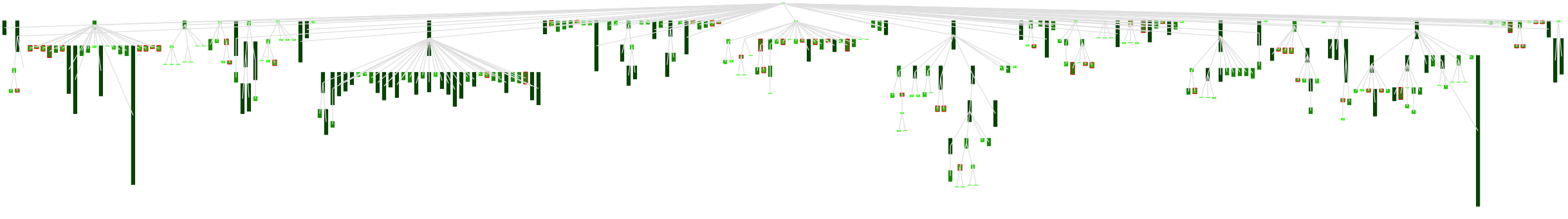 Right-click on the image and open it in a new window for a larger picture